Analysis

It is important to first discuss Merit number. While unrelated to the wick, finding the Merit number allows for selection of the proper working fluid. It was quite easy for us to go about selecting water as our working fluid given a plethora of prior research into the effective temperature ranges of various fluids. However, it remains important to justify each materials decision that was made at the beginning of the term by using established relationships and equations.

Merit number (N) equation

In this equation, p represents the liquid density, o the surface tension, h the latent heat, and u the viscosity of the fluid. A high liquid density and latent heat will allow the fluid to absorb more heat per unit volume, which will reduce the flow of fluid (and vapors) throughout the pipe needed to transfer a given amount of heat. A high surface tension will also allow the fluid to easily condense and flow back to the bottom of the pipe even at tight angled or horizontal orientations.

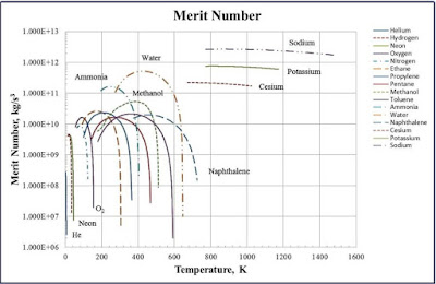
The Merit number is ultimately useful for determining the effective temperature range of each working fluid. By graphing a fluids merit number as a function of temperature, the following graph can be obtained.

www.1-act.com

The maximum of each curve is the temperature at which each fluid is most effective, meaning it can transfer the most amount of heat without completely vaporizing or condensing all of the fluid in the pipe. Since water is effective over the temperature range of 350K - 600K (170F - 620F), it will be best to use for the test rig, which will present temperatures towards the middle of this range.

We can also begin to describe the overall heat transfer capacity, or transfer power of the heat pipe. Given a working fluid operating in it's effective temperature range, the maximum amount of heat the pipe can transfer is given by

In this overall equation, there are several variables that need to be defined, assumed, and computed before continuing. o is the surface tension of the working fluid (water), which is dependent on temperature. This explains why a curve was formed above when the merit number was plotted as a function of temperature. Lt is the total length of the pipe, while Leff is the effective length of the pipe. During operation, it can be assumed that condensation and evaporation occur roughly halfway up the pipe, making Leff = 1/2Lt. y is the angle at which the heat pipe is tilted. This angle is formed with the horizontal. If the pipe were completely vertical, this angle would be 90, zeroing out the entire second term of the numerator.

The permeability (K_w) of each wick structure can be determined using the properties of a wick as shown in the equation below. D_sc is the diameter of the screen wire and φ is wick porosity.

Porosity (φ) is defined in the below equation, where W_sc is the length between adjacent wires.

The relationship between permeability and the overall fluid friction in the pipe can now be seen using the relationship described in the below proportion The original fluid friction equation has been simplified since all of our heat pipes are using the same working fluid (water), so its inherent properties of density and viscosity do not need to be accounted for.

We can now see that a relationship has emerged. The greater the permeability of the wick, the greater the internal fluid friction. Too much internal fluid friction reduces the quickness with which water can condense and be returned to the lower (heated) end of the pipe. It is important to try and reduce internal fluid friction.

We were able to calculate the permeability of the two wicks tested in our experiment using the above equations. We determined that K_w for the 22 hpi wick was 9.21x10^-4 mm² and K_w for the 16 hpi wick was 1.77x10^-3 mm².

This shows that the smaller, 22 hpi wick will have a lower fluid friction than the larger, 16 hpi wick. This justifies the results that we have obtained from the actual experiments.

The two graphs below represent the temperature of the pipe as a function of time. The blue line is the temperature at the heated end of the pipe and the orange line the temperature at the cooler end.

                          

By looking at only the curved portion of the graph, which represents the portion during which the working fluid was operating, we can use the below equation to find the rate of heat transfer in each trial. The blue line can be ignored since in both trials it leveled off to the same temperature, thus both trials were subject to the same conditions.

heat transfer rate = ΔT / Δt

For trial 1, consisting of the heat pipe with the 22 hpi wick, the average rate of heat transfer over the operational period was 0.085°F / s. Equilibrium was reached at a temperature of 102°F.

The same analysis was conducted for the 16 hpi wick in trial 2, using the curved portion from t = 390s to t = 600s. The average rate of heat transfer for this trial was 0.052°F / s over the operational period of the pipe. Equilibrium was established at a temperature of 92°F.

Thus, the relationship we have established is the smaller the wick size, the greater the rate of heat transfer. We have also saw that smaller wick sizes have less internal fluid friction. Our two results agree; smaller wick sizes create environments of lower fluid friction which in turn increase the rate at which heat is transferred from one end of the heat pipe to the other.

We conducted a third trial using the 22 hpi wick, which was the more effective of the two. However, we changed the amount of working fluid that was placed into the pipe to 35% of the total pipe volume. This allowed for greater efficiency of the heat pipe, as evidenced by the increased rate of heat transfer and nearly identical equilibrium temperatures at both ends of the pipe. The rate of heat transfer was taken from t = 390s to t = 780s and was calculated to be 0.136°F/s. The equilibrium temperatures were only 6°F apart from one another, indicating nearly maximum efficiency of the heat pipe.